XAS
Importing Dependencies
XSpecT relies on a number of common python packages including:
- h5py for reading HDF5 files
- NumPy and scipy for data analysis
- Matplotlib for visualization
- Other system related packages
Depending on your system you may need to install the necessary dependencies. S3DF users should have the necessary packages by default.
import h5py
import numpy as np
import matplotlib.pyplot as plt
from scipy.ndimage import rotate
from scipy.interpolate import interp1d
from scipy.optimize import curve_fit,minimize
import multiprocessing
import os
from functools import partial
import time
import sys
import argparse
from datetime import datetime
import tempfile
Importing XSPecT Modules
XSpecT has several main modules for function to control various aspects of the analysis, visualization, diagnostics and overall processing.
sys.path.insert(0, './XSpecT/')
import XSpect.XSpect_Analysis
import XSpect.XSpect_Controller
import XSpect.XSpect_Visualization
import XSpect.XSpect_PostProcessing
import XSpect.XSpect_Diagnostics
XAS Analysis Example
Setting up experiment parameters
Initializing the spectroscopy_experiment class and setting the relevant
experiment informationlslc_run, hutch, and experiment_id
parameters.
xas_experiment = XSpect.XSpect_Analysis.spectroscopy_experiment(lcls_run=22, hutch='xcs', experiment_id='xcsl1030422')
These values will be used to obtain the directory for the data which is
stored in experiment_directory:
'/sdf/data/lcls/ds/xcs/xcsl1030422/hdf5/smalldata'
XASBatchAnalysis Class
Instantiating the XASBatchAnalysis class which allows you to set
attributes relevant to the analysis such as the HDF5 group keys for the
various datasets, filter thresholds, and timing/energy parameters. The
class also contain an analysis pipeline method, which controls the
sequence of analysis operations.
Setting keys and aliases
The keys, which specify the data to read from the HDF5 file, are defined as a list of strings. For pump-probe XAS measurements this typically includes:
- The monochromator energy and set values (epics/ccm_E, epicsUser/ccm_E_setpoint)
- TT correction values and amplitude (tt/ttCorr, tt/AMPL)
- Timing stage values (epics/lxt_ttc)
- Emission CCD detecotr ROI sum values (epix_2/ROI_0_sum)
- Normalization channel (ipm4/sum).
Their "friendly" names serve as an easier to remember alias for the keys and are also defined as a list of strings with the same ordering as the keys.
These lists are passed to set_key_aliases which creates the key aliases.
keys=['epics/ccm_E', 'epicsUser/ccm_E_setpoint', 'tt/ttCorr', 'epics/lxt_ttc', 'enc/lasDelay', 'ipm4/sum', 'tt/AMPL', 'epix_2/ROI_0_sum']
names=['ccm', 'ccm_E_setpoint', 'time_tool_correction', 'lxt_ttc', 'encoder', 'ipm', 'time_tool_ampl', 'epix']
xas.set_key_aliases(keys,names)
Adding filters
Filters are set using add_filter which takes requires the parameters
\'shot_type\' (e.g. xray, simultaneous), \'filter_key\' (i.e. which
dataset to apply the filter to), and the filter threshold.
xas.add_filter('xray','ipm',500.0)
xas.add_filter('simultaneous','ipm',500.0)
xas.add_filter('simultaneous','time_tool_ampl',0.01)
Setting runs
Multiple runs (files) can be analyzed and combined into a single data set using the run_parser method.
Specify the runs as a list of strings or as a single string with space separated run numbers.
Ranges can be specified using numbers separated by a "-".
Setting timing parameters
Delay timing range and number of points is set in picoseconds.
Normalization option
Normalization is set by default (False) to use an IPM sum dataset. Alternatively, the scattering liquid ring signal can be used:
Running Analysis Loop
With the necessary parameters set the analysis procedure can be
initiatilized. Here you pass the experiment attributes from
xas_experiment. For details of the step by step analysis processes set
verbose= True (False is the default).
Obtained shot properties
HDF5 import of keys completed. Time: 0.02 seconds
Mask: xray has been filtered on ipm by minimum threshold: 500.000
Shots removed: 2645
Mask: simultaneous has been filtered on ipm by minimum threshold: 500.000
Shots removed: 1904
Mask: simultaneous has been filtered on time_tool_ampl by minimum threshold: 0.010
Shots removed: 100
Shots combined for detector epix on filters: simultaneous and laser into epix_simultaneous_laser
Shots (12182) separated for detector epix on filters: xray and laser into epix_xray_laser
Shots combined for detector ipm on filters: simultaneous and laser into ipm_simultaneous_laser
Shots (12182) separated for detector ipm on filters: xray and laser into ipm_xray_laser
Shots combined for detector ccm on filters: simultaneous and laser into ccm_simultaneous_laser
Shots (12182) separated for detector ccm on filters: xray and laser into ccm_xray_laser
Generated timing bins from -0.500000 to 2.000000 in 25 steps.
Generated ccm bins from 7.105000 to 7.156500 in 54 steps.
Shots combined for detector timing_bin_indices on filters: simultaneous and laser into timing_bin_indices_simultaneous_laser
Shots (12182) separated for detector timing_bin_indices on filters: xray and laser into timing_bin_indices_xray_laser
Shots combined for detector ccm_bin_indices on filters: simultaneous and laser into ccm_bin_indices_simultaneous_laser
Shots (12182) separated for detector ccm_bin_indices on filters: xray and laser into ccm_bin_indices_xray_laser
Detector epix_simultaneous_laser binned in time into key: epix_simultaneous_laser_time_energy_binned
Detector epix_xray_not_laser binned in time into key: epix_xray_not_laser_time_energy_binned
Detector ipm_simultaneous_laser binned in time into key: ipm_simultaneous_laser_time_energy_binned
Detector ipm_xray_not_laser binned in time into key: ipm_xray_not_laser_time_energy_binned
Obtained shot properties
HDF5 import of keys completed. Time: 0.03 seconds
...
Exploring Analyzed Runs
The data for each run is stored in analyzed_runs list.
[<XSpect.XSpect_Analysis.spectroscopy_run at 0x7febe6d2ea00>,
 <XSpect.XSpect_Analysis.spectroscopy_run at 0x7febe6de1d00>,
 <XSpect.XSpect_Analysis.spectroscopy_run at 0x7febe71fe580>,
 <XSpect.XSpect_Analysis.spectroscopy_run at 0x7febe6fab670>,
 <XSpect.XSpect_Analysis.spectroscopy_run at 0x7febe75ac550>,
 <XSpect.XSpect_Analysis.spectroscopy_run at 0x7febe75c4280>,
 <XSpect.XSpect_Analysis.spectroscopy_run at 0x7febe6fc07f0>,
 <XSpect.XSpect_Analysis.spectroscopy_run at 0x7febe6d2b1f0>,
 <XSpect.XSpect_Analysis.spectroscopy_run at 0x7febe6d2b460>,
 <XSpect.XSpect_Analysis.spectroscopy_run at 0x7febe6fb5e80>,
 <XSpect.XSpect_Analysis.spectroscopy_run at 0x7febe6fb53d0>,
 <XSpect.XSpect_Analysis.spectroscopy_run at 0x7febe6d2b9d0>,
 <XSpect.XSpect_Analysis.spectroscopy_run at 0x7febe6b00c10>,
 <XSpect.XSpect_Analysis.spectroscopy_run at 0x7febe72de340>]
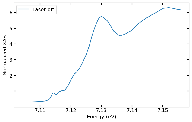
We can check the data shape for the laser-off shots first analyzed run, which has the dimensions of 25 time bins by 54 energy bins.
Data shape: (25, 54)
Since the laser the laser is off, we can average across all time bins for the epix and normalization channels.
y = np.average(xas.analyzed_runs[0].epix_xray_not_laser_time_energy_binned, axis = 0)
norm = np.average(xas.analyzed_runs[0].ipm_xray_not_laser_time_energy_binned, axis =0)
Plotting Laser-off Spectrum
Then the laser off spectrum can be plotted versus the monochromator energies.
plt.plot(xas.analyzed_runs[0].ccm_energies, y/norm, label="Laser-off")
plt.xlabel("Energy (eV)")
plt.ylabel("Normalized XAS")
plt.legend()
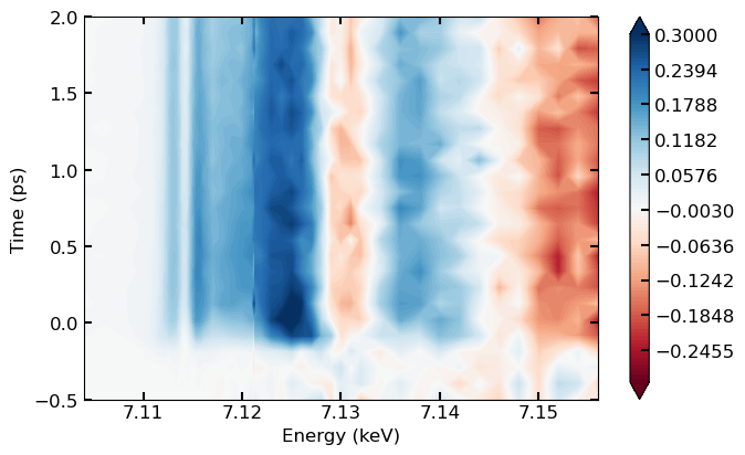
Plotting 2D Spectra
The 2D (time versus energy) data can be summed and plotted using the XSpecT visualation module.
First, from visualization the XASVisualization object is instantiated.
Then, using the combine_spectra method and passing the xas data object and the necessary data keys the data is processed.
v=XSpect.XSpect_Visualization.XASVisualization()
v.combine_spectra(xas_analysis=xas,
                  xas_laser_key='epix_simultaneous_laser_time_energy_binned',
                  xas_key='epix_xray_not_laser_time_energy_binned',
                  norm_laser_key='ipm_simultaneous_laser_time_energy_binned',
                  norm_key='ipm_xray_not_laser_time_energy_binned')
Finally, the 2D spectrum can be plotted, setting vmin and vmax colorbar parameters as needed.